Static, dynamic and continuous batching
GPUs are designed for highly parallel computation workloads, capable of performing trillions or even quadrillions of floating-point operations per second (FLOPs). Nevertheless, LLMs often fail to fully utilize these GPUs because much of the chip's memory bandwidth is spent loading model parameters.
Batching helps mitigate this bottleneck. In production, your service might be flooded with multiple requests arriving at the same time. Instead of processing each request individually, batching them together allows you to use the same loaded model parameters across multiple requests, thus dramatically improving throughput.
Use the simulator below to understand different batching strategies at a high level.
Static batching
The simplest form of batching is static batching. Here, the server waits until a fixed number of requests arrive and then processes them together as a single batch.
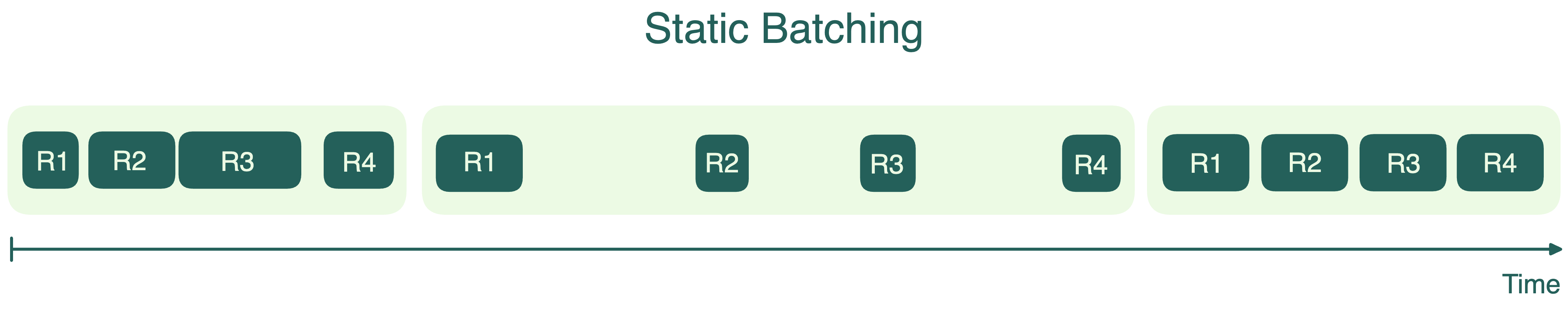
While static batching is easy to implement, it has notable downsides.
- The first request in a batch is forced to wait for the last one, adding unnecessary delay. Picture a printer that won’t start printing until you’ve queued up a set number of documents, regardless of how long it takes for the last document to arrive.
- Not all requests in a batch are created equal. In LLM inference, some requests may generate very short responses, while others could involve lengthy, step-by-step reasoning. Since all requests in the batch must wait until the slowest one finishes, this can lead to wasted compute resources and increased latency.
Dynamic batching
To address the issues in static batching, many systems use dynamic batching. This approach still collects incoming requests into batches, but it doesn’t insist on a fixed batch size. Instead, it sets a time window and processes whatever requests have arrived in that time frame. If the batch reaches its size limit sooner, it launches immediately. This is like a bus that leaves on a strict schedule or whenever it’s full, whichever happens first.
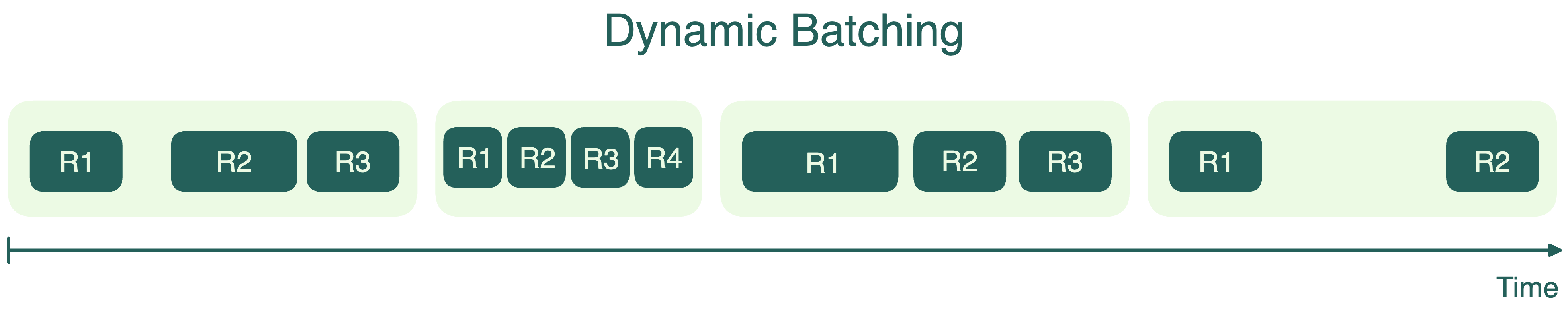
Dynamic batching helps balance throughput and latency. It ensures that early requests aren’t delayed indefinitely by later ones. However, because some batches might not be completely full when launched, it doesn’t always achieve maximum GPU efficiency. Another drawback is that, like static batching, the longest request in a batch still dictates when the batch finishes; short requests have to wait unnecessarily.
Continuous batching
For LLM inference, output sequences vary widely in length. Some users might ask simple questions, while others request detailed explanations. Static and dynamic batching force the short requests to wait for the longest one. This leaves GPU resources unsaturated.
Continuous batching, also known as in-flight batching, addresses these inefficiencies. Continuous batching doesn’t force the entire batch to complete before returning results. Instead, it lets each sequence in a batch finish independently and immediately replaces it with a new one. This is like an assembly line where, as soon as one item is finished (no matter how long it takes), a new item is added to keep the line running at full capacity.
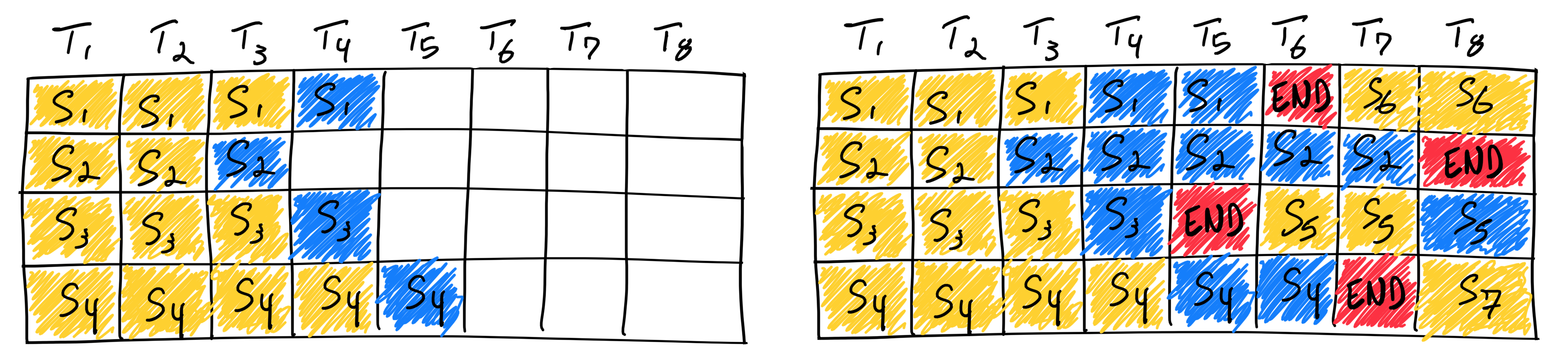
This technique uses iteration-level scheduling, meaning the batch composition changes dynamically at each decoding iteration. As soon as a sequence in the batch finishes generating tokens, the server inserts a new request in its place. This maximizes GPU occupancy and keeps compute resources busy by avoiding idle time that would otherwise be spent waiting for the slowest sequence in a batch to finish.
Major inference frameworks such as vLLM, SGLang, TensorRT-LLM (in-flight batching) and LMDeploy (persistent batching) all support continuous batching or similar mechanisms. For memory management in long or mixed-length batches, see PagedAttention.
FAQs
What are padding tokens in LLM batching?
Text sequences naturally have different lengths after tokenization. For example:
Sentence A: "Hello world"        # [15496, 995] - length 2
Sentence B: "How are you today?" # [2437, 389, 345, 1909] - length 4
You cannot directly stack these sequences into one dense rectangular tensor because their lengths differ. Padding solves this by adding placeholder tokens to shorter sequences so every request in the batch has the same tensor length. Common padding token forms include PAD, <pad>, or token ID 0, though the exact ID depends on the tokenizer.
An attention mask tells the model which positions are padding, but padding can still waste compute and memory. If a batch contains sequences with lengths like this:
[1024, 1000, 50, 20]
The shorter sequences may be padded to length 1024. That keeps the tensor shape regular for GPU kernels, but the 50-token and 20-token requests now carry a lot of unused positions.
What are ragged tensors in LLM inference?
Ragged tensors represent variable-length sequences without padding them all to one fixed length. Instead, the runtime stores the real tokens plus metadata such as sequence lengths, offsets, or KV cache block locations. This helps inference engines handle mixed-length prompts and continuous batching more efficiently, especially when paired with paged KV cache layouts such as PagedAttention.